What is a bill in Excel for NPOs and how can airSlate SignNow help?

A bill in Excel for NPOs refers to a financial document that details the expenses and payments for non-profit organizations. airSlate SignNow streamlines the process by allowing users to create, send, and eSign these invoices directly from Excel, ensuring that managing your billing is efficient and hassle-free.

How does airSlate SignNow handle eSigning for bills in Excel for NPOs?

With airSlate SignNow, you can easily integrate eSigning capabilities into your bills in Excel for NPOs. This allows your organization to get quick approvals, track signature statuses, and reduce delays in payment processing, all within a few clicks.

Are there any fees associated with creating a bill in Excel for NPOs using airSlate SignNow?

airSlate SignNow offers a range of pricing plans to fit your NPO’s budget. While creating and sending a bill in Excel for NPOs can be done at a low cost, check our pricing page for detailed information regarding subscription levels and any potential additional fees.

Can I customize the bills in Excel for NPOs with airSlate SignNow?

Yes, airSlate SignNow allows you to customize your bills in Excel for NPOs to reflect your brand's identity. You can modify templates, add your logo, and tailor the content to meet your specific needs and those of your stakeholders.

What are the benefits of using airSlate SignNow for bills in Excel for NPOs?

Using airSlate SignNow for bills in Excel for NPOs provides numerous benefits, including improved efficiency, quicker turnaround times for signatures, and enhanced tracking of billing documents. This ensures that your organization can focus more on its mission and less on administrative tasks.

Does airSlate SignNow integrate with accounting software for managing bills in Excel for NPOs?

Absolutely! airSlate SignNow integrates with various accounting software, making it easy to manage bills in Excel for NPOs seamlessly. This integration helps streamline your financial operations and ensures your billing records are always up to date.

Is it easy to train staff to use airSlate SignNow for creating bills in Excel for NPOs?

Definitely! airSlate SignNow is designed with user-friendliness in mind, so training your staff to create bills in Excel for NPOs is straightforward. Within a short time, your team will be able to navigate the platform and maximize its features efficiently.

Electronic Signature
Features
Invoice templates
Create a Bill in Excel for NPOs

Create a Bill in Excel for NPOs Effortlessly

Streamline your document management with airSlate SignNow's easy-to-use eSigning solution. Save time and reduce costs while enhancing your nonprofit's efficiency.

See how it works!Click here to sign a sample doc

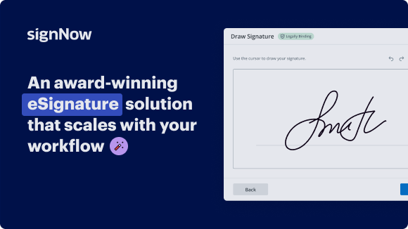
Award-winning eSignature solution

See airSlate SignNow eSignatures in action

Create secure and intuitive eSignature workflows on any device, track the status of documents right in your account, build online fillable forms – all within a single solution.

be ready to get more

Choose a better solution

Move your business forward with the airSlate SignNow eSignature solution

Create your signature in seconds on any desktop computer or mobile device, even while offline. Type, draw, or upload an image of your signature.

Deliver a seamless eSignature experience from any website, CRM, or custom app — anywhere and anytime.

Organize multiple documents in groups and automatically route them for recipients in a role-based order.

Collect signatures faster by sharing your documents with multiple recipients via a link — no need to add recipient email addresses.

Create unlimited templates of your most-used documents. Make your templates easy to complete by adding customizable fillable fields.

Create teams within airSlate SignNow to securely collaborate on documents and templates. Send the approved version to every signer.

Our user reviews speak for themselves

Kodi-Marie Evans

Director of NetSuite Operations at Xerox

airSlate SignNow provides us with the flexibility needed to get the right signatures on the right documents, in the right formats, based on our integration with NetSuite.

Check 5000+ reviews

Samantha Jo

Enterprise Client Partner at Yelp

airSlate SignNow has made life easier for me. It has been huge to have the ability to sign contracts on-the-go! It is now less stressful to get things done efficiently and promptly.

Check 5000+ reviews

Megan Bond

Digital marketing management at Electrolux

This software has added to our business value. I have got rid of the repetitive tasks. I am capable of creating the mobile native web forms. Now I can easily make payment contracts through a fair channel and their management is very easy.

Check 5000+ reviews

Collect signatures

24x

faster

Reduce costs by

$30

per document

Save up to

40h

per employee / month

airSlate SignNow solutions for better efficiency

Keep contracts protected

Enhance your document security and keep contracts safe from unauthorized access with dual-factor authentication options. Ask your recipients to prove their identity before opening a contract to bill in excel for npos.

Stay mobile while eSigning

Install the airSlate SignNow app on your iOS or Android device and close deals from anywhere, 24/7. Work with forms and contracts even offline and bill in excel for npos later when your internet connection is restored.

Integrate eSignatures into your business apps

Incorporate airSlate SignNow into your business applications to quickly bill in excel for npos without switching between windows and tabs. Benefit from airSlate SignNow integrations to save time and effort while eSigning forms in just a few clicks.

Generate fillable forms with smart fields

Update any document with fillable fields, make them required or optional, or add conditions for them to appear. Make sure signers complete your form correctly by assigning roles to fields.

Close deals and get paid promptly

Collect documents from clients and partners in minutes instead of weeks. Ask your signers to bill in excel for npos and include a charge request field to your sample to automatically collect payments during the contract signing.

be ready to get more

Why choose airSlate SignNow

Free 7-day trial. Choose the plan you need and try it risk-free.
Honest pricing for full-featured plans. airSlate SignNow offers subscription plans with no overages or hidden fees at renewal.
Enterprise-grade security. airSlate SignNow helps you comply with global security standards.

Start free trial

Your step-by-step guide — bill in excel for npos

Access helpful tips and quick steps covering a variety of airSlate SignNow’s most popular features.

Effective ways to create a bill in excel for NPOs

Creating a bill in Excel is essential for non-profit organizations (NPOs) to manage their finances efficiently. With the right tools, NPOs can streamline their billing processes, making it easier to track income and expenses. One such tool is airSlate SignNow, which offers a seamless e-signature experience to simplify document approvals.

Steps to create a bill in Excel for NPOs using airSlate SignNow

Open airSlate SignNow's website on your web browser.
Create an account for a free trial or log in if you already have one.
Upload the document you wish to sign or that needs signatures.
If you foresee using the same document again, convert it into a template.
Access the uploaded file and make necessary edits, such as adding fillable fields.
Sign your document and insert signature fields for your recipients.
Proceed by clicking Continue to finalize and dispatch an eSignature invitation.

In conclusion, leveraging airSlate SignNow not only simplifies the process of handling documents for NPOs but also enhances their operational efficiency. With its user-friendly interface and comprehensive features, organizations can achieve signNow cost savings and improved productivity.

Explore the benefits of airSlate SignNow today to optimize your document management processes!

How it works

Upload a document

Edit & sign it from anywhere

Save your changes and share

Connect airSlate SignNow to your apps

Check out airSlate SignNow integrations

Data accuracy, security, and compliance

airSlate SignNow is committed to protecting your sensitive information by complying with global industry-specific

Learn more about security

be ready to get more

Get legally-binding signatures now!

Start your free trial

FAQs

Here is a list of the most common customer questions. If you can’t find an answer to your question, please don’t hesitate to reach out to us.

Need help? Contact support

What active users are saying — bill in excel for npos

Get access to airSlate SignNow’s reviews, our customers’ advice, and their stories. Hear from real users and what they say about features for generating and signing docs.

This service is really great! It has helped...

5

anonymous

This service is really great! It has helped us enormously by ensuring we are fully covered in our agreements. We are on a 100% for collecting on our jobs, from a previous 60-70%. I recommend this to everyone.

Read full review

I've been using airSlate SignNow for years (since it...

5

Susan S

I've been using airSlate SignNow for years (since it was CudaSign). I started using airSlate SignNow for real estate as it was easier for my clients to use. I now use it in my business for employement and onboarding docs.

Read full review

Everything has been great, really easy to incorporate...

5

Liam R

Everything has been great, really easy to incorporate into my business. And the clients who have used your software so far have said it is very easy to complete the necessary signatures.

Read full review