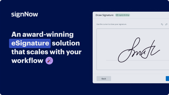
Collaborate on Billing Statement in Excel for Quality Assurance with Ease Using airSlate SignNow

Billing statement in excel for Quality Assurance

Hi everyone, Kevin here. Today I want to show you how you can create  an interactive dashboard in Microsoft Excel. With a dashboard, you can showcase the most  important information to your organization,   and best of all, it's actually really easy to  set up. You don't have to know any VBA and you   don't have to any add-ins. All you  need is the base version of Microsoft Excel. Once you finish creating your  dashboard, as new data comes in,   it'll automatically update  to reflect the latest data. Also, once you're ready to share it out  with other people in your organization,   you can very easily share it so they  can get insights from your dashboard. If you want to follow along today, I've included  a sample spreadsheet in the description. All right, let's check this out. Here I am in Microsoft Excel, and I  want to create a performance dashboard   for the Kevin Cookie Company.  Leadership is always asking me   questions about things like our profit,  unit sales, and that type of business stuff. Now I figured I could create a dashboard  to answer all of those different questions. That way I can continue  focusing on my YouTube videos. As you can see, I don't have  anything in this workbook yet,   but luckily, I have data to build my dashboard.  Down below, let's click on the data worksheet.   On the data sheet, here you'll see sales  data by market for the Kevin Cookie Company. Now keep in mind this is internal data, but  I figured it would serve as a good example. So just between you and me, keep it on the  down low that I shared this sheet with you. To build our dashboard, we're  going to create a few pivot tables. This table that you see here is  currently in a tabular format   and this works really well  for creating pivot tables. If you're new to pivot tables, I've included  an overview video in the description. Also, even if you're not new to pivot  tables, I've also included a link to   a video that covers some of the more  advanced aspects of pivot tables, and   if you think you know pivot tables, trust  me, there's always something new to learn. I'm learning new things about them all the time. As a first step, we need to make sure that our  data here is in a table format. To turn it into   a table, simply click anywhere in your data and  then go up to the top ribbon and click on insert. Right here you have the option  to turn it into a table. You can also press the shortcut key Control + T. Let's click on this. In this prompt, it  asks me for where my data is, and here it   automatically identified all of the different  data that I want to bring into this table. Here it also asks me if my table has headers,  and this is my header right up here, it does,   so I'll make sure that I check this box. Next, let's click on OK. All of my data is now included in a table,  and it has this nice table formatting. Next, I want to insert a pivot table. So once again, I'll click into my table and  then up on the top ribbon, let's click on   insert and all the way over on the left-hand  side, there’s the option to insert a pivot table. When you click on that, that opens up a prompt and  it asks us what table or range do we want to use? I'll simply select this Table 3. This is the table that I just created. I'll place my pivot table on a new  worksheet, and then I'll click on   OK. This now drops me into a new worksheet, sheet  1, and I can now start building my pivot table.   For my dashboard, I want to  have three different charts,   so I'm going to need three different pivot  tables and right now I only have one. If I go down below over to all of my  different sheets, I can press the control key,   click on sheet 1, and then drag it over. This will create another pivot table. It's just a copy of sheet one. Here I'll press the control  key again, click on this sheet,   drag it over, and now I have  three different pivot tables   and I’ll use these three different sheets to  pull together all of my views for my dashboard. The first view I want to pull together  is profit by country and cookie. Here I'll right click on this tab,   and I'll select rename and let me call this  just what it is, profit by country and cookie. Now that I've renamed the sheet, I'm ready  to pull together my first pivot table,   and once again, I want to know  profit by country and cookie type.   Over on the right-hand side, I have  all of my different pivot table fields. First, I'll select country and  I'll pull that down into rows.   Here we can see all of the different countries  that we operate in for the Kevin Cookie Company. Also, over on the right-hand side,  I see a field called product. Here I'll drag that down to columns, and  here you can see all of the different   cookies that we make here, and trust  me, they're all extremely delicious. Over here I'll select profit, bring it  down into values, and here I can see all   of our different countries, all of the  cookie types, and the associated profit. Now that I see all of my data here, I  want to make a few formatting changes. Right now, you see that it  doesn't show up as a currency. Here I'll select all of these different values. I'll click up on home up above, and here,  let me turn on the currency formatting type. Also, I don't need all of  these different decimals. I know, every penny counts, but for this analysis  it's not necessary. Here I'll remove the decimals. Before I insert a chart to  visually show this data,   I want to make one more tweak to the pivot table. I want to make sure that I show all of  the different markets in order of most   profitable to least profitable, and I want to  do the same for the different cookie types. Here I'll zoom out just a little bit and  I'll click into the grand total column. Here I'll right click, I'll go over to sort,  and I'll sort from largest to smallest. So here you see that India  is our most profitable market   and the United States is the least profitable. Thank you to all of the Indian  viewers of this channel,   we've been able to achieve record profits. We can now do the same for  the different cookie types. Over here I'll right click, go down to sort, and  I'll sort this from largest to smallest as well. So now the markets are sorted from the most  profitable to least, and same with the cookies. Now that my pivot table is all done,   I'm ready to insert a chart and we're  going to use this chart on our dashboard. To insert a chart, let's go to the top  tabs and click on pivot table analyze. Over on the right-hand side, there's  the option to insert a pivot chart. Let's click on that. This opens up the insert chart dialog, and right  here I'm going to select the stacked column chart. Next, let's click on OK. And here now you can see a pivot  chart representing all of this data. Now when we did this sorting here, here  you'll see all of the different markets   are sorted from the largest over on the left  all the way down to the smallest on the right. Also, with the stacked bar chart, here  you'll notice that the largest items are   at the bottom and the smallest items are at the  top, so it makes it easier to consume the data. Overall this looks pretty good, but  I think I need a title on this chart   just so when people look at it,  they can understand what it is. Let's go up to the top tabs, click on design,  and all the way over on the left-hand side,   click on add chart elements. Right here we'll go down to chart title and I'll  add it above the chart. For the chart title,   I'll simply describe what it is. It's profit by market and cookie type. Before I bring this chart back to my  dashboard, I want to clean up a few   things. Here I have all of these different  field items included on my chart.   Here if I click on this, I can filter my product,  but I don't want this cluttering up my chart.   Here I could right click on the item,  and I'll select to remove or hide   all field buttons on this chart, and when  I select that, it really helps clean it up. I'm now ready to move this chart to my dashboard.   Here I'll select the chart  and I'll press Control + C. Next, I'll click over to my dashboard,  and I'll paste it onto this sheet. And check that out, I now have  my first visual on my dashboard.   Here I'll zoom out just a little bit so  I can see how it sits on my dashboard. Here I can select the chart item, and  if I press the alt key at the same time,   it'll snap into different positions. So, this way I can organize my  dashboard a little bit more easily. Here I'll position this first item right here  and I'll extend it down just a little bit,   maybe right down to this point.  I think that looks pretty good. Next, I want to create two more  pivot tables for my dashboard,   and I'll do these a little bit more quickly. Down below, I'll click on the next sheet, and here  I'll rename this, and we'll call this units sold   each month. To track units sold each month, here  I'll select the date and I'll make this my row,   and right up here, I'll select  units sold as the values. So here I could see by month  how many units we sold.   To help with the formatting, here  I'll highlight all of the numbers,   and I'll insert the comma style, and  I'll also remove the decimal points. Just like we did before, I'll click on  pivot table analyze, and here I'll insert   a pivot chart. For unit sales over time, I  think a line chart will work really well. I’ll select this one and then click on OK. This now inserts my chart and here I'll  update the title to say units sold each month. Here I'll remove the legend, and I want to  remove the fields just like I did before. Here I'll right click, and I’ll  hide all field buttons on the chart. This now looks really good, so I'll copy  it and I'll bring it into my dashboard. In my dashboard, I'll press control + V to paste   and here I'll position it right near the top,  and here I'll reduce the size just a little bit. That looks pretty good. Lastly, I want to create one more  pivot table for my dashboard. I'll go down to the bottom tabs and let  me rename this one to profit by month.   To create a pivot table with profit by month,  it's going to be very similar to the last pivot   table that we created. Here I'll select  months and I'll drag it down into rows. Next, I'll select profit and  I'll pull it down into values. And here we see our profit by month. Like I've always said, there is  money in the cookie business. Next I want to set it so it appears as a currency. I'll highlight all of these values and  here I’ll select the currency view. Also, I'll remove the decimal places. Next  I want to insert a chart, so once again,   I'll click on the tab titled Pivot Table analyze  and right here I'll select a pivot chart.   To represent data over time,  line charts work very well. Here I'll select line and then I'll click on OK. This now inserts my chart, and I don't know  why profit decreased in November and December. Those are the holidays, we  should be reaching records. I'm sure management will be  interested in this. Right up here,   I'll click on the title of the chart,  and I'll put in profit by month. I'll click over on the legend that  says total and here I'll delete that,   and just like we did before, I want  to remove all of the different fields. I think that'll make the dashboard look better. Once again, I'll right click and  select hide all field buttons on chart. Next, I want to bring this chart over to my  dashboard, so once again, I'll select the chart,   press control + C to copy, and  then I'll click into my dashboard. Here within the dashboard,  I'll press control + V to paste   and here all position it under units sold  each month, and I'll make my best attempt   at trying to make it just about the  same size. Now just like we did before,   I can press the Alt key and then this  item will snap to the cells on the page. Here I'll do the same down here and now everything  lines up nicely. To make sure everything aligns   very nicely on this page, I have a few different  alignment tools. Here I'll select this chart,   I'll select this one, and I'll go up  to the top tabs called shape format. Over on the right-hand side, here I have  my alignment tools and here I'll make   sure that I align them to the top and  they were already aligned at the top,   but if they weren't, that  would help me achieve that. Next, I'll select these two  different charts right down here. Once again, I'll go to shape format  and let me align them to the left,   so these are also in alignment with one another. So, everything looks nice and  organized. Along with setting   alignment, I could also specify the  exact dimensions of one of these charts. Here also like this chart and  I'll go up to format up on top,   and over here I can see the  precise height and width,   so I could adjust these if I want different  charts to be the exact same height and width. So far, we just have a static dashboard and I want  to make sure that people can interact with this   dashboard. To make it dynamic, let's select one of  the items, and then go up to pivot chart analyze. On this ribbon, there's the option to  insert slicers and also a timeline. First, let's insert a timeline.  Within the timeline prompt,   I'll select a date and then  click on OK. This inserts a   timeline slicer. Here I'll select the item,  and I'll drag it over to the left-hand side,   and here I'll adjust the dimensions, so  it sits right alongside different items. Next, I want to insert some additional slicers. Once again, I'll select this pivot  table, I'll go up to pivot chart analyze,   and over here, I’ll select insert slicer. Within this dialog, I'll select  both country and product. I want to quickly be able to filter my  data by the country and the product. Next, I'll click on OK. This now inserts two slicers, but before  I bring it over to the left-hand side,   I want to clean them up a little bit. When you look at this list, it's pretty  obvious that these are all countries,   so I don't need this header that says country. Here I'll right click on the  item, I'll select slicer settings,   and I'll turn off the display  header, then I'll click on OK. I'll do the same for product. Now that  neither of these items have a header,   here I'll resize it, so it just  fits the different slicer items. I'll do the same over here. Now I can  drag this slicer over onto the side. I'll position it right here and I'll  do the same with the product type. With this slicers over on the left-hand side,   you'll notice that the  width is not quite the same. Here I can select this first item, I'll click  on timeline and here I can see the width. I'll set it to two   and all select these other items, and  all set the same width for them as well. Here now you can see that they  all have the exact same width.   With my slicers now in place, I can very  quickly filter the data on my dashboard. Let's say for example, I just  want to see data for India. Here I could select India and you'll  notice that my profit only shows India,   but my two other views didn't update. How can I make sure that  these slicers are connected to   all of the different pivot tables?  Here I'll right click on the slicer,   and let's go down to report connections. Within  report connections, I can specify what pivot   tables this slicer controls, and currently it's  only set to the profit by market and cookie type. I want to make sure it updates all of my  different pivot tables, so here I'll check   all of these boxes and then click on OK. I’ll  do the same for the other two slicers as well. And check this out! When I click on my slicers  now, it updates all of my different pivot   tables over on this side, so this dashboard is  definitely becoming a lot more interactive now.   Let's take a look at chocolate chip cookies in the  US. Look at that, I can see how much profit for   that cookie type. If I want to select multiple  items with a slicer, here I can simply click   on India and then drag my mouse down and that'll  select all of these different markets and here I   could do the same for the product, so it's very  easy to look at my data how I want to view it. This dashboard is working really well,   but what new data comes in and we want to  make sure that our dashboard reflects it?   Well, it's very easy to take care of. Down  below, let's click into the new data tab and   here you'll see that we have additional data for  2020. It’s formatted in exactly the same format. Here let's select all the data from  this table and then press control + C. Once you copy all of the data,  let's click into the data sheet,   and go all the way to the bottom of the table. This is the table that we used to  construct all of our pivot tables,   and here simply paste in all of the new data. Because we turned this into a table,   it automatically incorporates this  new data into that same table. Next, on the bottom, let's  click back into our dashboard,   and we want to make sure that the dashboard  now reflects all of the latest data. To do that, let's click into one of these pivot  charts and then go up to pivot chart analyze. Within the ribbon here,  there's the option to refresh. Let's click on this and then select  refresh all. And there you'll see   that your dashboard automatically takes  all of the latest data into account. This dashboard now is starting to look pretty  nice, but it still has the look and feel of Excel,   and I want it to look more like  a proper dashboard. To do that,   let's go up to the view tab up on top, and with  the sheets selected right here, you have the   option to turn off the gridlines, so there you  don't have those typical cells in Excel. Also,   here I can turn off the headings, so now it's  really starting to feel more like a dashboard. Also, down below, we have all  of these separate sheets for   all the different pivot tables and the data. Here I could select all of those different sheets,   I could right click, and then I  could hide those different sheets.   So now if you share this sheet out, people will  only see the dashboard that you pulled together. This dashboard is now starting  to look really nice, but maybe   the color scheme doesn't match your organization. Well, that's no problem. We can also change that.   Up on top with the top tabs, click on the one  titled page layout and over on the left-hand side,   you can choose from all of these different  themes and that'll apply it to your dashboard. Also, within themes, you can even browse  for other themes, or you could even save   a theme that you create, so you can customize  this to look exactly how you want it to look.   Now that we've created the dashboard and  it looks exactly how you want it to look,   you probably want to share it out with  other people in your organization.   Up in the top right-hand corner,  you can click on the share icon. This opens up the share dialog, and here  you could decide whether people can edit   the sheet or if it's only view only. Back  here, you can select people you want to   share it with, or you can simply  copy a link and then share it out. All right, well, let me know down below in the  comments, were you able to successfully create   a dashboard? To see more videos like this, please  consider subscribing, and I'll see you next time.