What is the bilty format in excel for nonprofit organizations?

The bilty format in excel for nonprofit organizations refers to a structured template designed to record and manage shipping and logistics details. By using an effective bilty format, nonprofits can streamline their operational processes and ensure better tracking of their goods and services.

How can airSlate SignNow help with the bilty format in excel for nonprofit?

airSlate SignNow offers tools that enable nonprofit organizations to create, send, and eSign documents in the bilty format in excel for nonprofit. This can signNowly simplify the process of managing shipping logistics while ensuring compliance and reducing the potential for errors.

Is there a cost associated with using airSlate SignNow for bilty format in excel for nonprofit?

Yes, airSlate SignNow provides various pricing plans to accommodate different sizes of nonprofit organizations. You can choose a plan that best fits your needs, including features tailored specifically for managing documents in the bilty format in excel for nonprofit.

What features does airSlate SignNow offer for creating the bilty format in excel for nonprofit?

airSlate SignNow includes features such as customizable templates, real-time collaboration, and automated workflows that can support the creation of the bilty format in excel for nonprofit. These functionalities make it easier for nonprofits to maintain organized records of their shipments.

Can airSlate SignNow integrate with other software I use for managing the bilty format in excel for nonprofit?

Absolutely! airSlate SignNow offers seamless integrations with various software tools commonly used by nonprofit organizations, allowing for easy data sharing and enhanced workflow efficiency when working with the bilty format in excel for nonprofit.

What are the benefits of using airSlate SignNow for nonprofits dealing with the bilty format in excel?

Using airSlate SignNow provides nonprofits with a more efficient way to handle documents in the bilty format in excel. Benefits include improved accuracy, faster processing times, and easier compliance with legal requirements, allowing nonprofits to focus on their core mission.

How does airSlate SignNow ensure the security of the bilty format in excel for nonprofit?

airSlate SignNow prioritizes security by implementing advanced encryption technology for all documents, including those in the bilty format in excel for nonprofit. This ensures that sensitive information remains protected and only accessible to authorized users.

Electronic Signature
Features
Invoice templates
Bilty Format in Excel for Nonprofit

Discover the Best Bilty Format in Excel for Nonprofit Organizations

Streamline your document management with airSlate SignNow's user-friendly eSigning solution. Save time and reduce costs while effectively managing your nonprofit's paperwork.

See how it works!Click here to sign a sample doc

Award-winning eSignature solution

See airSlate SignNow eSignatures in action

Create secure and intuitive eSignature workflows on any device, track the status of documents right in your account, build online fillable forms – all within a single solution.

be ready to get more

Choose a better solution

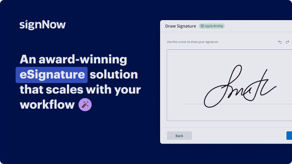
Move your business forward with the airSlate SignNow eSignature solution

Create your signature in seconds on any desktop computer or mobile device, even while offline. Type, draw, or upload an image of your signature.

Deliver a seamless eSignature experience from any website, CRM, or custom app — anywhere and anytime.

Organize multiple documents in groups and automatically route them for recipients in a role-based order.

Collect signatures faster by sharing your documents with multiple recipients via a link — no need to add recipient email addresses.

Create unlimited templates of your most-used documents. Make your templates easy to complete by adding customizable fillable fields.

Create teams within airSlate SignNow to securely collaborate on documents and templates. Send the approved version to every signer.

Our user reviews speak for themselves

Kodi-Marie Evans

Director of NetSuite Operations at Xerox

airSlate SignNow provides us with the flexibility needed to get the right signatures on the right documents, in the right formats, based on our integration with NetSuite.

Check 5000+ reviews

Samantha Jo

Enterprise Client Partner at Yelp

airSlate SignNow has made life easier for me. It has been huge to have the ability to sign contracts on-the-go! It is now less stressful to get things done efficiently and promptly.

Check 5000+ reviews

Megan Bond

Digital marketing management at Electrolux

This software has added to our business value. I have got rid of the repetitive tasks. I am capable of creating the mobile native web forms. Now I can easily make payment contracts through a fair channel and their management is very easy.

Check 5000+ reviews

Collect signatures

24x

faster

Reduce costs by

$30

per document

Save up to

40h

per employee / month

airSlate SignNow solutions for better efficiency

Keep contracts protected

Enhance your document security and keep contracts safe from unauthorized access with dual-factor authentication options. Ask your recipients to prove their identity before opening a contract to bilty format in excel for nonprofit.

Stay mobile while eSigning

Install the airSlate SignNow app on your iOS or Android device and close deals from anywhere, 24/7. Work with forms and contracts even offline and bilty format in excel for nonprofit later when your internet connection is restored.

Integrate eSignatures into your business apps

Incorporate airSlate SignNow into your business applications to quickly bilty format in excel for nonprofit without switching between windows and tabs. Benefit from airSlate SignNow integrations to save time and effort while eSigning forms in just a few clicks.

Generate fillable forms with smart fields

Update any document with fillable fields, make them required or optional, or add conditions for them to appear. Make sure signers complete your form correctly by assigning roles to fields.

Close deals and get paid promptly

Collect documents from clients and partners in minutes instead of weeks. Ask your signers to bilty format in excel for nonprofit and include a charge request field to your sample to automatically collect payments during the contract signing.

be ready to get more

Why choose airSlate SignNow

Free 7-day trial. Choose the plan you need and try it risk-free.
Honest pricing for full-featured plans. airSlate SignNow offers subscription plans with no overages or hidden fees at renewal.
Enterprise-grade security. airSlate SignNow helps you comply with global security standards.

Start free trial

Your step-by-step guide — bilty format in excel for nonprofit

Access helpful tips and quick steps covering a variety of airSlate SignNow’s most popular features.

How to create a bilty format in excel for Nonprofit organizations

Creating a bilty format in Excel for nonprofits can streamline your documentation processes and improve efficiency. With airSlate SignNow, you can manage your e-signature needs seamlessly, allowing for quicker approvals and enhanced productivity.

Steps to create a bilty format in excel for Nonprofit organizations using airSlate SignNow

Open your preferred web browser and navigate to the airSlate SignNow homepage.
Create an account with a complimentary trial or log in if you already have an account.
Select the document you need for signing or choose to upload a new one.
If you envision using this document repeatedly, transform it into a reusable template.
Access your uploaded file to make necessary modifications: incorporate fillable fields or add relevant data.
Finalize your document by adding your signature and including signature fields for recipients.
Proceed by clicking 'Continue' to configure and dispatch an eSignature invitation.

Using airSlate SignNow offers various advantages such as an excellent return on investment due to its comprehensive feature set relative to cost, user-friendly design suitable for SMBs and Mid-Market businesses, transparent pricing without unexpected fees, and reliable 24/7 support provided with all premium subscriptions.

Embrace the advantages of electronic signatures today and elevate your nonprofit's operational efficiency—sign up for your free trial now!

How it works

Access the cloud from any device and upload a file

Edit & eSign it remotely

Forward the executed form to your recipient

Connect airSlate SignNow to your apps

Check out airSlate SignNow integrations

Data accuracy, security, and compliance

airSlate SignNow is committed to protecting your sensitive information by complying with global industry-specific

Learn more about security

be ready to get more

Get legally-binding signatures now!

Start your free trial

FAQs

Here is a list of the most common customer questions. If you can’t find an answer to your question, please don’t hesitate to reach out to us.

Need help? Contact support

What active users are saying — bilty format in excel for nonprofit

Get access to airSlate SignNow’s reviews, our customers’ advice, and their stories. Hear from real users and what they say about features for generating and signing docs.

This service is really great! It has helped...

5

anonymous

This service is really great! It has helped us enormously by ensuring we are fully covered in our agreements. We are on a 100% for collecting on our jobs, from a previous 60-70%. I recommend this to everyone.

Read full review

I've been using airSlate SignNow for years (since it...

5

Susan S

I've been using airSlate SignNow for years (since it was CudaSign). I started using airSlate SignNow for real estate as it was easier for my clients to use. I now use it in my business for employement and onboarding docs.

Read full review

Everything has been great, really easy to incorporate...

5

Liam R

Everything has been great, really easy to incorporate into my business. And the clients who have used your software so far have said it is very easy to complete the necessary signatures.

Read full review