What is a commission bill format in Excel for human resources?

A commission bill format in Excel for human resources is a structured spreadsheet that helps HR departments calculate and record commission payments for employees. This format can streamline the commission calculation process, ensuring accuracy and efficiency in payroll management.

How can airSlate SignNow help with the commission bill format in Excel for human resources?

airSlate SignNow facilitates the eSigning of commission bill formats in Excel for human resources, allowing for seamless and secure document handling. It ensures that all necessary approvals are captured quickly, improving workflow efficiency and minimizing delays in processing commission payments.

Is the commission bill format in Excel compatible with other software?

Yes, the commission bill format in Excel for human resources can be easily integrated with various HR software solutions. This compatibility allows HR teams to import and export data effortlessly, ensuring a smooth transition of information across different platforms.

What features does airSlate SignNow offer for managing commission bill formats?

airSlate SignNow offers robust features for managing commission bill formats in Excel for human resources, including customizable templates and automatic workflows. These features help HR professionals save time and reduce errors when processing commission bills and obtaining necessary approvals.

How does using a commission bill format in Excel benefit HR departments?

Using a commission bill format in Excel for human resources standardizes the commission tracking process, improving overall accuracy and accountability. It also allows for easier reporting and analysis, enabling HR departments to quickly assess commission trends and make data-driven decisions.

Can I try airSlate SignNow for free to manage my commission bill formats?

Yes, airSlate SignNow offers a free trial that allows you to explore its features for managing commission bill formats in Excel for human resources. This trial provides a risk-free opportunity to see how the solution can enhance your document management and eSigning processes.

What types of businesses can benefit from a commission bill format in Excel?

Any business that utilizes commission payments can benefit from a commission bill format in Excel for human resources. This includes sales organizations, real estate firms, and service-based companies, all of which can leverage the format to streamline payroll and enhance operational efficiency.

Electronic Signature
Features
Invoice templates
Commission Bill Format in Excel for Human Resources

Unlock the Perfect Commission Bill Format in Excel for Human Resources

Streamline your HR processes with airSlate SignNow's easy-to-use eSigning solution. Save time and reduce costs while ensuring secure document management.

See how it works!Click here to sign a sample doc

Award-winning eSignature solution

See airSlate SignNow eSignatures in action

Create secure and intuitive eSignature workflows on any device, track the status of documents right in your account, build online fillable forms – all within a single solution.

be ready to get more

Choose a better solution

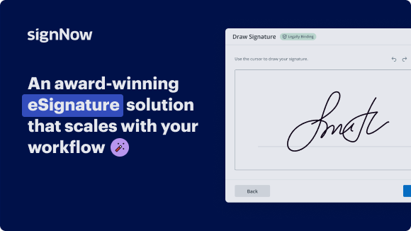
Move your business forward with the airSlate SignNow eSignature solution

Create your signature in seconds on any desktop computer or mobile device, even while offline. Type, draw, or upload an image of your signature.

Deliver a seamless eSignature experience from any website, CRM, or custom app — anywhere and anytime.

Organize multiple documents in groups and automatically route them for recipients in a role-based order.

Collect signatures faster by sharing your documents with multiple recipients via a link — no need to add recipient email addresses.

Create unlimited templates of your most-used documents. Make your templates easy to complete by adding customizable fillable fields.

Create teams within airSlate SignNow to securely collaborate on documents and templates. Send the approved version to every signer.

Our user reviews speak for themselves

Kodi-Marie Evans

Director of NetSuite Operations at Xerox

airSlate SignNow provides us with the flexibility needed to get the right signatures on the right documents, in the right formats, based on our integration with NetSuite.

Check 5000+ reviews

Samantha Jo

Enterprise Client Partner at Yelp

airSlate SignNow has made life easier for me. It has been huge to have the ability to sign contracts on-the-go! It is now less stressful to get things done efficiently and promptly.

Check 5000+ reviews

Megan Bond

Digital marketing management at Electrolux

This software has added to our business value. I have got rid of the repetitive tasks. I am capable of creating the mobile native web forms. Now I can easily make payment contracts through a fair channel and their management is very easy.

Check 5000+ reviews

Collect signatures

24x

faster

Reduce costs by

$30

per document

Save up to

40h

per employee / month

airSlate SignNow solutions for better efficiency

Keep contracts protected

Enhance your document security and keep contracts safe from unauthorized access with dual-factor authentication options. Ask your recipients to prove their identity before opening a contract to commission bill format in excel for human resources.

Stay mobile while eSigning

Install the airSlate SignNow app on your iOS or Android device and close deals from anywhere, 24/7. Work with forms and contracts even offline and commission bill format in excel for human resources later when your internet connection is restored.

Integrate eSignatures into your business apps

Incorporate airSlate SignNow into your business applications to quickly commission bill format in excel for human resources without switching between windows and tabs. Benefit from airSlate SignNow integrations to save time and effort while eSigning forms in just a few clicks.

Generate fillable forms with smart fields

Update any document with fillable fields, make them required or optional, or add conditions for them to appear. Make sure signers complete your form correctly by assigning roles to fields.

Close deals and get paid promptly

Collect documents from clients and partners in minutes instead of weeks. Ask your signers to commission bill format in excel for human resources and include a charge request field to your sample to automatically collect payments during the contract signing.

be ready to get more

Why choose airSlate SignNow

Free 7-day trial. Choose the plan you need and try it risk-free.
Honest pricing for full-featured plans. airSlate SignNow offers subscription plans with no overages or hidden fees at renewal.
Enterprise-grade security. airSlate SignNow helps you comply with global security standards.

Start free trial

Your step-by-step guide — commission bill format in excel for human resources

Access helpful tips and quick steps covering a variety of airSlate SignNow’s most popular features.

Commission bill format in excel for Human Resources

Creating an efficient commission bill format in Excel for Human Resources can streamline your payroll process. By utilizing tools like airSlate SignNow, you can simplify document signing and management, ensuring that all necessary approvals are obtained swiftly and securely.

Steps to use airSlate SignNow effectively

Navigate to the airSlate SignNow website in your web browser.
Create a new account for a free trial or log into your existing account.
Select and upload the document you wish to sign or need to send for signatures.
If you anticipate using this document again, convert it into a reusable template.
Open the uploaded document to make necessary edits: add fillable fields or insert specific information.
Add your own signature and include signature fields for other recipients.
Click 'Continue' to configure and send out an eSignature invitation.

In conclusion, airSlate SignNow provides an invaluable tool that allows businesses to manage document signatures efficiently and at a lower cost. With its user-friendly interface and transparent pricing, it's designed to fit the needs of small to mid-sized businesses.

Get started today and transform your document signing process!

How it works

Open & edit your documents online

Create legally-binding eSignatures

Store and share documents securely

Connect airSlate SignNow to your apps

Check out airSlate SignNow integrations

Data accuracy, security, and compliance

airSlate SignNow is committed to protecting your sensitive information by complying with global industry-specific

Learn more about security

be ready to get more

Get legally-binding signatures now!

Start your free trial

FAQs

Here is a list of the most common customer questions. If you can’t find an answer to your question, please don’t hesitate to reach out to us.

Need help? Contact support

What active users are saying — commission bill format in excel for human resources

Get access to airSlate SignNow’s reviews, our customers’ advice, and their stories. Hear from real users and what they say about features for generating and signing docs.

amazing

5

User in Insurance

What do you like best?

Obviously I like the fact that during this COVID time I don't have to risk my health by going to meet people in person and that everything is done online.

Read full review

Excellent Product!

5

Administrator in Hospital & Health Care

What do you like best?

Easy to navigate, the ability to create multiple templates.

Read full review

airSlate SignNow Review

5

User in Internet

What do you like best?

very easy and convenient to use, best app we've used this quarantine