What is an hourly invoice template for product management in Google Docs?

An hourly invoice template in Google Docs for product management is a structured document that allows you to easily track billable hours and expenses for projects. It simplifies the invoicing process, enabling product managers to create professional invoices quickly, enhancing both productivity and clarity in billing.

How can I customize the hourly invoice template for product management in Google Docs?

You can easily customize the hourly invoice template for product management in Google Docs by editing text, adding your company logo, and modifying the layout to fit your branding needs. This flexibility allows you to create a personalized invoice that reflects your business, ensuring a professional presentation to your clients.

Is the hourly invoice template for product management free to use?

Yes, the hourly invoice template for product management in Google Docs is free to use. This cost-effective solution makes it accessible for businesses of all sizes, allowing you to create and send invoices without worrying about software costs.

What features does the hourly invoice template for product management include?

The hourly invoice template for product management includes features such as fields for billable hours, a breakdown of services, tax calculations, and payment terms. These features are designed to streamline your invoicing process, making it easier to manage and track payments.

Can I integrate the hourly invoice template for product management with other tools?

Yes, the hourly invoice template for product management in Google Docs can be integrated with various tools such as Google Drive and accounting software. This integration helps streamline workflows by allowing you to access, share, and manage invoices efficiently across platforms.

How does using an hourly invoice template for product management benefit my business?

Using an hourly invoice template for product management can signNowly benefit your business by saving time and reducing errors during the billing process. It ensures that clients receive clear and accurate invoices, which can enhance cash flow and improve client satisfaction.

What are the best practices for using an hourly invoice template for product management?

Best practices for using an hourly invoice template for product management include clearly listing billable hours, providing a detailed description of services rendered, and setting clear payment terms. Ensuring clarity in your invoices helps prevent misunderstandings and fosters good client relationships.

Electronic Signature
Features
Invoice templates
Hourly Invoice Template Google Docs for Product Management

Collaborate on Hourly Invoice Template Google Docs for Product Management with Ease Using airSlate SignNow

Watch your billing procedure become quick and effortless. With just a few clicks, you can perform all the required actions on your hourly invoice template google docs for Product Management and other crucial files from any device with web connection.

See how it works!Click here to sign a sample doc

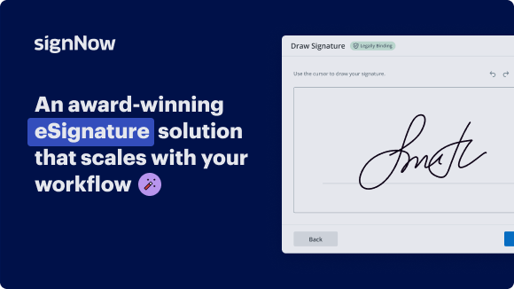
Award-winning eSignature solution

See airSlate SignNow eSignatures in action

Create secure and intuitive eSignature workflows on any device, track the status of documents right in your account, build online fillable forms – all within a single solution.

be ready to get more

Choose a better solution

Move your business forward with the airSlate SignNow eSignature solution

Create your signature in seconds on any desktop computer or mobile device, even while offline. Type, draw, or upload an image of your signature.

Deliver a seamless eSignature experience from any website, CRM, or custom app — anywhere and anytime.

Organize multiple documents in groups and automatically route them for recipients in a role-based order.

Collect signatures faster by sharing your documents with multiple recipients via a link — no need to add recipient email addresses.

Create unlimited templates of your most-used documents. Make your templates easy to complete by adding customizable fillable fields.

Create teams within airSlate SignNow to securely collaborate on documents and templates. Send the approved version to every signer.

Our user reviews speak for themselves

Kodi-Marie Evans

Director of NetSuite Operations at Xerox

airSlate SignNow provides us with the flexibility needed to get the right signatures on the right documents, in the right formats, based on our integration with NetSuite.

Check 5000+ reviews

Samantha Jo

Enterprise Client Partner at Yelp

airSlate SignNow has made life easier for me. It has been huge to have the ability to sign contracts on-the-go! It is now less stressful to get things done efficiently and promptly.

Check 5000+ reviews

Megan Bond

Digital marketing management at Electrolux

This software has added to our business value. I have got rid of the repetitive tasks. I am capable of creating the mobile native web forms. Now I can easily make payment contracts through a fair channel and their management is very easy.

Check 5000+ reviews

Collect signatures

24x

faster

Reduce costs by

$30

per document

Save up to

40h

per employee / month

airSlate SignNow solutions for better efficiency

Keep contracts protected

Enhance your document security and keep contracts safe from unauthorized access with dual-factor authentication options. Ask your recipients to prove their identity before opening a contract to hourly invoice template google docs for product management.

Stay mobile while eSigning

Install the airSlate SignNow app on your iOS or Android device and close deals from anywhere, 24/7. Work with forms and contracts even offline and hourly invoice template google docs for product management later when your internet connection is restored.

Integrate eSignatures into your business apps

Incorporate airSlate SignNow into your business applications to quickly hourly invoice template google docs for product management without switching between windows and tabs. Benefit from airSlate SignNow integrations to save time and effort while eSigning forms in just a few clicks.

Generate fillable forms with smart fields

Update any document with fillable fields, make them required or optional, or add conditions for them to appear. Make sure signers complete your form correctly by assigning roles to fields.

Close deals and get paid promptly

Collect documents from clients and partners in minutes instead of weeks. Ask your signers to hourly invoice template google docs for product management and include a charge request field to your sample to automatically collect payments during the contract signing.

be ready to get more

Why choose airSlate SignNow

Free 7-day trial. Choose the plan you need and try it risk-free.
Honest pricing for full-featured plans. airSlate SignNow offers subscription plans with no overages or hidden fees at renewal.
Enterprise-grade security. airSlate SignNow helps you comply with global security standards.

Start free trial

Your step-by-step guide — hourly invoice template google docs for product management

Access helpful tips and quick steps covering a variety of airSlate SignNow’s most popular features.

Explore how to ease your workflow on the hourly invoice template google docs for Product Management with airSlate SignNow.

Looking for a way to simplify your invoicing process? Look no further, and adhere to these simple steps to conveniently collaborate on the hourly invoice template google docs for Product Management or request signatures on it with our easy-to-use service:

Set up an account starting a free trial and log in with your email credentials.
Upload a file up to 10MB you need to sign electronically from your device or the web storage.
Continue by opening your uploaded invoice in the editor.
Perform all the required steps with the file using the tools from the toolbar.
Press Save and Close to keep all the changes performed.
Send or share your file for signing with all the needed addressees.

Looks like the hourly invoice template google docs for Product Management workflow has just turned more straightforward! With airSlate SignNow’s easy-to-use service, you can easily upload and send invoices for eSignatures. No more generating a printout, signing by hand, and scanning. Start our platform’s free trial and it simplifies the whole process for you.

How it works

Open & edit your documents online

Create legally-binding eSignatures

Store and share documents securely

Connect airSlate SignNow to your apps

Check out airSlate SignNow integrations

Data accuracy, security, and compliance

airSlate SignNow is committed to protecting your sensitive information by complying with global industry-specific

Learn more about security

be ready to get more

Get legally-binding signatures now!

Start your free trial

FAQs

Here is a list of the most common customer questions. If you can’t find an answer to your question, please don’t hesitate to reach out to us.

Need help? Contact support

What active users are saying — hourly invoice template google docs for product management

Get access to airSlate SignNow’s reviews, our customers’ advice, and their stories. Hear from real users and what they say about features for generating and signing docs.

Great App

5

Administrator in Construction

What do you like best?

I like the fact that we can easily send a document that requires a signature a get it back quickly and making it shareable with a group of people.

Read full review

airSlate SignNow helped bring our business to the next level

5

Administrator in Leisure, Travel & Tourism

What do you like best?

airSlate SignNow was easy to use as well as easy for our customers.

Read full review

airSlate SignNow is awesome and easy to use!

5

Rachel Presser

What do you like best?

It’s easy to upload files and the overall UX is easy to use. I like the variety of fields, it makes sending contracts simple, especially the invitations for signers—gives my clients a great impression!

Read full review