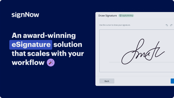
Collaborate on Import Invoice Format for Finance with Ease Using airSlate SignNow

Import invoice format for Finance

Today, let's talk about a very useful Excel  tool that will help you clean up your data. Now,   this is especially helpful if you work  in accounting because, as an accountant,   you probably find yourself downloading data from  other systems like SAP, Oracle, and the like,   and you need to clean these up to be able to  prepare your reports. So, the tool that I'm going   to show you is like a magic box; it can do a lot  and it doesn't require that much effort from you.   I thought the best way of introducing this to you  is with practical examples, so let's get to it. Let's take a look at the data that we need to  import into Excel and analyze. We have an SAP   extract which comes from our European entity; it's  the income statement. But take a look at this:   our numbers are all over the place; they're not  even recognized as numbers because the data is   coming from Europe. It's using a dot for the  thousand separator and a comma for the decimal   place. Now they're also not properly aligned in a  column. We have a lot of information here that we   don't need and a lot of gaps in our data. We need  to bring this to Excel and clean it up and our aim   is not just to clean this up, but also to get a  report that looks like this. We want to get the   current year-to-date information for revenue,  expenses and profit and loss and compare this   to last year. And in case we need the details,  we want to get them properly here so that it's   easier for us to analyze the numbers. Now, what  would happen if you just copy this information   and paste it into Excel? Let's try it. I'm  going to press Ctrl+A to select everything,   Ctrl+C. Let's go back to our sheet here and let's  create a new tab and Ctrl+V. This is how it's   going to look: our numbers are still problematic.  We also have a lot of white space in front of some   of these numbers. And take a look at this: here  we have "main revenue"; there is no number here,   the number is showing up in the next column and  we have a third column here. Sometimes it looks   like the numbers show up in the third column. For  the majority of the cases, they are in the first   column. Now, this information here is for the  current period, so that's the reporting period,   and this is the comparison period. It looks like  we have the same issue where some of the numbers   are in the second column and sometimes they might  go to the third column. Now, this last column here   is the absolute difference, so that's just going  to be the difference between these two numbers.   For our analysis, we're not really going to need  the absolute difference because we can make that   calculation easily in Excel. Now, how do we clean  this up though? Well, in Excel, you have different   options. From the Data tab you have features  like Text to Columns, Remove Duplicates. You   have functions like the TRIM function or  SEARCH and REPLACE to clean up this data.   If we're going to be honest, this is going to  take us a lot of manual work and if this is a   task we have to repeat on a frequent basis, it's  going to cost us a lot of time every single time.   Now, instead of using the tools available on  this side, I'm going to use the tools available on   this side because this way, I get to save the  steps I do so that every time I get new data,   everything will be updated automatically the  moment I press Refresh. Now, before I get there,   let's just quickly take a look at the way we would  clean up this data set. If I scroll to the left,   there are a lot of columns that I don't need.  So the first few columns here, until the income   statement, I don't need those. I would be able to  get rid of them. I also have some complete empty   rows here which I can get rid of. The next two  columns also look empty, we can just double check.   There isn't much there except this semicolon.  This one also looks empty, so I'm just pressing   Ctrl+down and Ctrl+up to take a look. There isn't  anything there that we want to keep. Then we have   the description, this is something we definitely  want to keep, followed by our numbers here. Now   for the numbers, we have a few things to solve. We  have to combine them into one column and translate   them into numbers that our Excel understands.  This Excel here uses US regional settings. Okay, so now that we're clear on the type of  cleanup we need to do, let's go ahead and do   this. I'm going to delete this, and now let's go  and explore the left side. Get and Transform,   our SAP data is in a text file. So From Text/CSV, the file I want to import is sitting in my   C drive, it's in the Info folder, and that's the  file. Just select it and click on import. Here,   I get to see a preview of my file. We know that  we have to do a lot of transformations here,   so we're not going to load this directly.  Instead, we're going to transform the data. Now we're inside the Power Query Editor.  Here, we can choose the different types   of transformations we want to do. We can  give our final result, so the final table,   a different name. I'm going to call it  'Clean Data'. And here are Applied Steps,   so any steps that we do to clean up the data is  going to be recorded and remembered. So, anytime   our source changes, the steps will automatically  apply whenever we refresh our final report. In   case the name of your source file changes or the  location of the file changes, you can click on the   gear icon and browse for your file, or just update  the name directly in here and then click on OK. Now Power Query went ahead and applied a 'Changed  Type' step here, so that it defines the type of   data that's inside a column. I was thinking  that pretty much everything is a text column,   but that's not the case, right? We have a lot of  numbers here, so we need to update that. But it's   too early to update it. We're going to do it later  when we have proper column headers. So, I'm just   going to remove that step. First, let's go and  take care of our numbers here. So, remember we   had the issue that sometimes the number was here,  and sometimes it was even in the third column like   in this case. We want to bring this number to this  column and this number as well in here. For this,   I can use 'Merge'. Select this column, hold down  Shift, select column 13, right-mouse-click 'Merge   Columns', separator is none because I either  have something in the cell or I don't. The new   column name, let's call this 'Current Period'  and OK. Everything is now merged in one column. Next, we need to repeat this for the previous  year, which is these three columns here.   So, I'm going to select, hold  down Shift, select column 16,   right-mouse-click, 'Merge Columns', leave separator  as none, call this 'Previous Year Period'.   Now, let's get rid of the columns that we don't  need. Actually, in fact, since the columns that we   want to keep are less than what we want to get rid  of, let's just pick the ones that we want to keep.   I want to keep the income statement and the  descriptions. So, this time I'm going to hold   down Control, select column eight. The first  set of numbers here are my current period,   and the second one is the previous year  period, so you have to ignore this.   We're going to get rid of these in a second.  I don't need anything else from this. So, with   the columns that I've highlighted, I'm going to  right-mouse-click and remove other columns. Okay,   so far so good. I don't need all these rows here.  Let's remove them, remove rows, remove top rows   10. I'm going to remove all the way up to here  and, okay, now things are starting to look better.   I have these empty rows that I can get rid of, so  let's go and filter them out by removing the blank   rows here and OK. Now notice, anytime we add  a new step, we can see Power Query writing these   steps, writing these functions for us. It's always  good to keep an eye on these, so even if you   don't really understand them, make sure that you  can see these steps. In case you don't see it,   go to the View tab and activate the formula bar.  So, in case yours is not activated, you're not   going to see those steps. Place a checkmark here  so you can follow these along. Okay, so now, let's   take care of these numbers. If I just go and  change the type of this column to a currency,   it's not going to work, so let's remove the step.  Instead, we have to tell it what's the origin of   this number. Now, since our issue is with this  one and this one, I'm just going to select them   both, then right-mouse-click, 'Change Type', and go  to "Using Locale." Here I can define the origin   of this number. The data type I want is going  to be currency. The locale here is not English,   so let's scroll down until we get to German,  and we have German (Austria). When I select that,   I can see a preview of how the original number  should look like. In this case, it doesn't look   like that because it has the dot here as a  thousand separator. So, instead of Austria,   let's go with Germany, that's the number that  I'm dealing with. So, now let's click on OK,   and everything is properly transformed. This is  a text column, this one is a text column as well,   so I'm going to leave that as is. Now, one thing  I noticed here is I have the colon after the text,   and since in my final report I don't have these,  I'm just going to remove them. Select a column,   go to Home, Replace Values, look for "colon"  and replace it with nothing and click on OK.   This step is recorded as well, so everything  that we did got recorded. Anytime we need to   make a correction to this, or include a step in  between steps, we can go and do that. There's one   last thing I need to do here, give these proper  names and I'm done. So, let's test this out, Close   and Load, Close and Load To. We can load it as a  table on a new worksheet, but in this case, I'll   just put it on the side here. So, I'll go with  existing worksheet and let's go with F1 and OK.   Our data is clean. Now if, at this stage, you  notice some things that you want to remove,   you can always go and edit your query. So, you can  just double-click here, go back to the query, and   add a step. For example, I can remove the bottom  rows, I don't want that last row, so I'm going to   put 'one,' and 'OK,' and then just click on 'Close  and Load,' and it's going to refresh the existing   query. So now that last row has disappeared.  In addition to cleaning up the accounts,   we also want to create our summary report. We  have all the information that we need from here,   all we have to do is use a function and  grab what we need. Because in this case,   the labels are identical to what I have in my  source data, I can do a direct lookup on this.   In case you have different labels, you can use  a helper column as your identifier. The type   of lookup function you're going to use here is  going to depend on your version of Excel because   if you have Excel for Office 365, you're probably  going to want to use the new 'XLOOKUP' function,   which is easier to use than 'VLOOKUP.' If you have  other versions of Excel, 'VLOOKUP' will work. Our   lookup value is this value right here, the table  array is our table, so I'm just going to go to the   side to select it. The column index number we want  to return is the third column, that's where we   have the current period, so I'm going to put a three.  Last argument is if I want an approximate match   or an exact match. Well, I want an exact match, I  can either go with 'false' or put a zero in here,   close bracket, press Enter, and I have my  value. Now, I need to reverse the sign here   because revenue in the system is a credit,  so I have to reverse the sign for these.   Now, just so that I can copy this and also paste  it to the next column, I'm going to be mindful of   my cell referencing for 'A4.' Let's fix the column  reference, the rest remains the same because   I'm using table references. Now, let me also go  and update the number formatting and remove the   decimal places. OK, so revenue total will be  from here, material, and services total as well,   so are these. So, I'll just do these in  one go. I'm going to hold down 'CTRL,'   select them, and then press 'CTRL + V' to paste in  my formula. Next, let's calculate the percentages.   Here, I want to take material and divide this with  revenue. Now again, I'm going to be mindful of the   cell references because I want to be able to copy  it, not just down, but also to the next column. So,   for revenue here, let's press 'F4' two times. So,  this time I'm keeping the row fixed but the column   dynamic. This reference remains dynamic, so that  every time I'm going to be referencing the cell   above the percentage. Let's adjust the formatting  to a percentage and copy these to the other cells.   Now, that I've done everything for this column,  let's just copy the whole column, paste it here.   There is some part that we need to change  because instead of getting the third column,   we want to return the fourth column. I'll just do  a quick replacement here, highlight these cells,   press 'CTRL + H,' I'm gonna look for 'comma  three,' 'comma zero,' just to make sure I'm   in the right part of the formula and  replace it with 'four,' replace all,   OK, and we're done. The great thing about  this process is when I get new data because   all I have to do is refresh this. So let's say I  get a new file, I'm just going to grab that file   and drop it in the same location as I have the  previous file, they have the same name, so I'm   going to replace the file in the destination.  Now I just need to go back to my report,   right-mouse-click and refresh. Now, keep your eyes  on column B data. All the steps run automatically   and I get the latest data. Now, in case your file  has a different name or is in a different folder,   you can just go back to your query, go to  the Source step, click on the gear icon and   update the file from here. Click on OK,  Close and Load, and your report is done. Before we wrap up, I want to show you another  example. What if our data is in Excel and we   need to create a pivot table from it? So in this  case, I have account, date, transaction number,   supplier, and amount and I want to create a pivot  table with amount per supplier. In this case, I'm   just dealing with sample data, but imagine I had  a lot of this. If I was cleaning this up manually,   it's going to take me a lot of time, so I'm  going to use Power Query instead. First thing,   I'm going to do is transform this into an Excel  table, so let's press Ctrl + T and see what range   is picked up. It just thinks that this is our  data set because we have gaps in the data,   so let's correct that and select our sample  here. My data has headers, click on OK.   Under Table Design, let's update the name of  our table and let's also remove the table style   to go back to the previous style we had before.  In case you want to remove these drop-downs here,   uncheck Filter Button. So everything looks like  it did originally. Now that this is a table and   we have a proper name for it, go to Data, From  Table Range, and send this to Power Query. We can   remove the Changed Type step at this point and add  it later on. To clean this data, I want to remove   any of these rows where I just have no values.  So I'm going to click on this drop-down here and   uncheck Null and OK. So everything that doesn't  equal to null is included. Next, let's filter out   the totals because if I leave them in there, the  pivot table is just going to include them as data.   I need to get rid of them, let's use text  filters, 'does not equal' and type in "TOTAL".   So Power Query is case sensitive, I  have to be mindful of that and OK. Next,   let's fill these down. I need to have an account  for each row, so I'm going to right-mouse-click,   Fill, Down. Now, what I'd also like to do is to  remove the code here. There are different ways   I can approach this depending on your data set and  what is consistent in your data set. In this case,   I can go to Transform, Split Column, and go with  something like 'By Digit to Non-Digit.' This is   going to give me multiple columns and then I can  get rid of this if I always have just three digits,   or I can also base it on the number of characters.  So in this case, I'll go to Split Column and use   'By Number of Characters.' "Specify the number  of characters used to split the text column."   So I have one, two, three, four, five and six,  including the space. I want to split this once   as far left as possible and OK. The split is  done. Power Query thought that   these are dates. I don't even need this at all,  so I'm just going to press delete and remove it.   Let's rename this column to "Account". Now,  we can take care of the column types. This   is a text column; I want this to be a  date only. This can be a whole number. "Supplier" is text, and "Amount"  is currency. Everything is done.   Let's update the name of our end pivot table  and call it "Clean Report". Now, go to File,   Close and Load To, this time, I want it as a pivot  table report. Let's put it in the existing sheet   and I'll put it right here on the side, and OK.  Put "Amount" in the values field and "Supplier" in   the rows field, and let's take a look. We have our  pivot table. Let's update the number formatting.   Right-mouse-click, number format, use a  thousand separator, and zero decimal places. Now, because it's a pivot table we can look at  this in any way we want. We can also add "Account"   and "Supplier" here or just put "Account" as  the filter. Anytime our data source updates,   we just need to refresh this to get the latest  information. I hope this video gave you some ideas   on how you can use Power Query to clean up your  data. Now, there is a lot that Power Query can do,   and I have a complete course about it, in case  you want to go deeper. Thank you for being here.   Thank you for watching till the end. If you're new  here, don't forget to hit that subscribe button,   give this video a thumbs up, and  I'll see you in the next video.