What is a bills template Google Sheets for operations?

A bills template Google Sheets for operations is a pre-designed spreadsheet that helps businesses manage their invoicing and billing processes efficiently. It allows users to customize fields, track expenses, and streamline their financial operations, enhancing productivity and accuracy.

How can I use the bills template Google Sheets for operations?

You can use the bills template Google Sheets for operations by downloading it and customizing it to fit your specific needs. Simply input your company's information, add the necessary data for each bill, and utilize built-in formulas to track expenses and calculate totals seamlessly.

Is the bills template Google Sheets for operations easy to integrate with other tools?

Yes, the bills template Google Sheets for operations is designed to work well with various applications, such as airSlate SignNow, for document signing and management. This integration allows you to send invoices and receive electronic signatures directly from your spreadsheet, streamlining your workflow.

What are the pricing options for airSlate SignNow when using a bills template Google Sheets for operations?

airSlate SignNow offers competitive pricing plans that cater to businesses of all sizes. When using a bills template Google Sheets for operations, you can choose a plan that best fits your needs, ensuring that you have access to essential features without overspending.

What features should I look for in a bills template Google Sheets for operations?

Look for features such as customizable fields, automatic calculations, and easy data entry when selecting a bills template Google Sheets for operations. Additional functionality, like integration with airSlate SignNow for seamless e-signatures, can signNowly improve your billing process.

What are the benefits of using a bills template Google Sheets for operations?

Using a bills template Google Sheets for operations brings numerous benefits, including enhanced efficiency, reduced errors, and better control over your financial data. It simplifies record-keeping and can improve cash flow management by providing clear visibility into billing and expenses.

Can I customize the bills template Google Sheets for operations?

Absolutely! The bills template Google Sheets for operations is fully customizable, allowing you to adjust columns, headings, and formulas to meet your specific business requirements. This flexibility ensures that you can create a billing solution that aligns with your operational needs.

Electronic Signature
Features
Invoice templates
Bills Template Google Sheets for Operations

Collaborate on Bills Template Google Sheets for Operations with Ease Using airSlate SignNow

See your billing procedure turn quick and effortless. With just a few clicks, you can perform all the required actions on your bills template google sheets for Operations and other important documents from any gadget with web connection.

See how it works!Click here to sign a sample doc

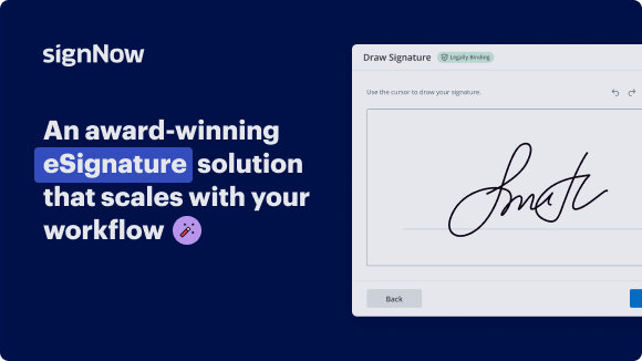
Award-winning eSignature solution

See airSlate SignNow eSignatures in action

Create secure and intuitive eSignature workflows on any device, track the status of documents right in your account, build online fillable forms – all within a single solution.

be ready to get more

Choose a better solution

Move your business forward with the airSlate SignNow eSignature solution

Create your signature in seconds on any desktop computer or mobile device, even while offline. Type, draw, or upload an image of your signature.

Deliver a seamless eSignature experience from any website, CRM, or custom app — anywhere and anytime.

Organize multiple documents in groups and automatically route them for recipients in a role-based order.

Collect signatures faster by sharing your documents with multiple recipients via a link — no need to add recipient email addresses.

Create unlimited templates of your most-used documents. Make your templates easy to complete by adding customizable fillable fields.

Create teams within airSlate SignNow to securely collaborate on documents and templates. Send the approved version to every signer.

Our user reviews speak for themselves

Kodi-Marie Evans

Director of NetSuite Operations at Xerox

airSlate SignNow provides us with the flexibility needed to get the right signatures on the right documents, in the right formats, based on our integration with NetSuite.

Check 5000+ reviews

Samantha Jo

Enterprise Client Partner at Yelp

airSlate SignNow has made life easier for me. It has been huge to have the ability to sign contracts on-the-go! It is now less stressful to get things done efficiently and promptly.

Check 5000+ reviews

Megan Bond

Digital marketing management at Electrolux

This software has added to our business value. I have got rid of the repetitive tasks. I am capable of creating the mobile native web forms. Now I can easily make payment contracts through a fair channel and their management is very easy.

Check 5000+ reviews

Collect signatures

24x

faster

Reduce costs by

$30

per document

Save up to

40h

per employee / month

airSlate SignNow solutions for better efficiency

Keep contracts protected

Enhance your document security and keep contracts safe from unauthorized access with dual-factor authentication options. Ask your recipients to prove their identity before opening a contract to bills template google sheets for operations.

Stay mobile while eSigning

Install the airSlate SignNow app on your iOS or Android device and close deals from anywhere, 24/7. Work with forms and contracts even offline and bills template google sheets for operations later when your internet connection is restored.

Integrate eSignatures into your business apps

Incorporate airSlate SignNow into your business applications to quickly bills template google sheets for operations without switching between windows and tabs. Benefit from airSlate SignNow integrations to save time and effort while eSigning forms in just a few clicks.

Generate fillable forms with smart fields

Update any document with fillable fields, make them required or optional, or add conditions for them to appear. Make sure signers complete your form correctly by assigning roles to fields.

Close deals and get paid promptly

Collect documents from clients and partners in minutes instead of weeks. Ask your signers to bills template google sheets for operations and include a charge request field to your sample to automatically collect payments during the contract signing.

be ready to get more

Why choose airSlate SignNow

Free 7-day trial. Choose the plan you need and try it risk-free.
Honest pricing for full-featured plans. airSlate SignNow offers subscription plans with no overages or hidden fees at renewal.
Enterprise-grade security. airSlate SignNow helps you comply with global security standards.

Start free trial

Your step-by-step guide — bills template google sheets for operations

Access helpful tips and quick steps covering a variety of airSlate SignNow’s most popular features.

Explore how to streamline your workflow on the bills template google sheets for Operations with airSlate SignNow.

Searching for a way to simplify your invoicing process? Look no further, and follow these quick steps to conveniently work together on the bills template google sheets for Operations or request signatures on it with our easy-to-use service:

Сreate an account starting a free trial and log in with your email credentials.
Upload a file up to 10MB you need to sign electronically from your PC or the web storage.
Continue by opening your uploaded invoice in the editor.
Take all the required steps with the file using the tools from the toolbar.
Select Save and Close to keep all the changes performed.
Send or share your file for signing with all the necessary addressees.

Looks like the bills template google sheets for Operations process has just turned simpler! With airSlate SignNow’s easy-to-use service, you can easily upload and send invoices for eSignatures. No more printing, manual signing, and scanning. Start our platform’s free trial and it optimizes the entire process for you.

How it works

Open & edit your documents online

Create legally-binding eSignatures

Store and share documents securely

Connect airSlate SignNow to your apps

Check out airSlate SignNow integrations

Data accuracy, security, and compliance

airSlate SignNow is committed to protecting your sensitive information by complying with global industry-specific

Learn more about security

be ready to get more

Get legally-binding signatures now!

Start your free trial

FAQs

Here is a list of the most common customer questions. If you can’t find an answer to your question, please don’t hesitate to reach out to us.

Need help? Contact support

What active users are saying — bills template google sheets for operations

Get access to airSlate SignNow’s reviews, our customers’ advice, and their stories. Hear from real users and what they say about features for generating and signing docs.

This service is really great! It has helped...

5

anonymous

This service is really great! It has helped us enormously by ensuring we are fully covered in our agreements. We are on a 100% for collecting on our jobs, from a previous 60-70%. I recommend this to everyone.

Read full review

I've been using airSlate SignNow for years (since it...

5

Susan S

I've been using airSlate SignNow for years (since it was CudaSign). I started using airSlate SignNow for real estate as it was easier for my clients to use. I now use it in my business for employement and onboarding docs.

Read full review

Everything has been great, really easy to incorporate...

5

Liam R

Everything has been great, really easy to incorporate into my business. And the clients who have used your software so far have said it is very easy to complete the necessary signatures.

Read full review