What is a hardware bill format for education?

A hardware bill format for education outlines the specifications, costs, and quantities of hardware items required for educational purposes. This format helps schools and educational institutions effectively budget and procure the necessary hardware while ensuring compliance with regulations and standards.

Why is implementing a hardware bill format for education important?

Implementing a hardware bill format for education is crucial for streamlining procurement processes and avoiding budget overruns. It ensures transparency and accountability in spending while facilitating better planning and alignment with educational goals.

How does airSlate SignNow enhance the hardware bill format for education?

airSlate SignNow enhances the hardware bill format for education by providing a digital signing solution that simplifies document approval processes. Users can seamlessly create, send, and eSign hardware bills, making the procurement process faster and more efficient.

What features does airSlate SignNow offer for managing hardware bills?

airSlate SignNow offers features such as customizable templates for hardware bills, real-time document tracking, and secure eSigning. These features help educational institutions streamline their workflows while ensuring that the hardware bill format for education meets compliance standards.

Can I integrate airSlate SignNow with other educational software?

Yes, airSlate SignNow offers integrations with various educational software and platforms, making it easy to incorporate the hardware bill format for education into existing workflows. This flexibility allows schools to maintain their preferred systems while enhancing document management.

What are the pricing options for airSlate SignNow?

airSlate SignNow offers competitive pricing plans tailored to the needs of educational institutions, which include features related to the hardware bill format for education. Plans are structured to accommodate various user levels, ensuring that schools get the best value for their investment.

How does eSigning a hardware bill format for education enhance security?

ESigning a hardware bill format for education through airSlate SignNow enhances security by employing encryption, audit trails, and authentication measures. These features protect sensitive information and ensure that only authorized individuals can approve hardware purchases.

Electronic Signature
Features
Invoice templates
Hardware Bill Format for Education

Collaborate on Hardware Bill Format for Education with Ease Using airSlate SignNow

See your invoicing process become fast and effortless. With just a few clicks, you can complete all the necessary actions on your hardware bill format for Education and other important files from any gadget with internet access.

See how it works!Click here to sign a sample doc

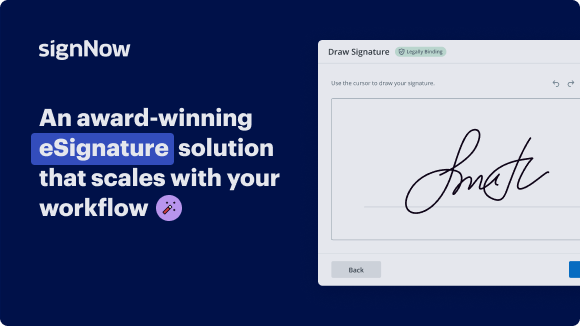
Award-winning eSignature solution

See airSlate SignNow eSignatures in action

Create secure and intuitive eSignature workflows on any device, track the status of documents right in your account, build online fillable forms – all within a single solution.

be ready to get more

Choose a better solution

Move your business forward with the airSlate SignNow eSignature solution

Create your signature in seconds on any desktop computer or mobile device, even while offline. Type, draw, or upload an image of your signature.

Deliver a seamless eSignature experience from any website, CRM, or custom app — anywhere and anytime.

Organize multiple documents in groups and automatically route them for recipients in a role-based order.

Collect signatures faster by sharing your documents with multiple recipients via a link — no need to add recipient email addresses.

Create unlimited templates of your most-used documents. Make your templates easy to complete by adding customizable fillable fields.

Create teams within airSlate SignNow to securely collaborate on documents and templates. Send the approved version to every signer.

Our user reviews speak for themselves

Kodi-Marie Evans

Director of NetSuite Operations at Xerox

airSlate SignNow provides us with the flexibility needed to get the right signatures on the right documents, in the right formats, based on our integration with NetSuite.

Check 5000+ reviews

Samantha Jo

Enterprise Client Partner at Yelp

airSlate SignNow has made life easier for me. It has been huge to have the ability to sign contracts on-the-go! It is now less stressful to get things done efficiently and promptly.

Check 5000+ reviews

Megan Bond

Digital marketing management at Electrolux

This software has added to our business value. I have got rid of the repetitive tasks. I am capable of creating the mobile native web forms. Now I can easily make payment contracts through a fair channel and their management is very easy.

Check 5000+ reviews

Collect signatures

24x

faster

Reduce costs by

$30

per document

Save up to

40h

per employee / month

airSlate SignNow solutions for better efficiency

Keep contracts protected

Enhance your document security and keep contracts safe from unauthorized access with dual-factor authentication options. Ask your recipients to prove their identity before opening a contract to hardware bill format for education.

Stay mobile while eSigning

Install the airSlate SignNow app on your iOS or Android device and close deals from anywhere, 24/7. Work with forms and contracts even offline and hardware bill format for education later when your internet connection is restored.

Integrate eSignatures into your business apps

Incorporate airSlate SignNow into your business applications to quickly hardware bill format for education without switching between windows and tabs. Benefit from airSlate SignNow integrations to save time and effort while eSigning forms in just a few clicks.

Generate fillable forms with smart fields

Update any document with fillable fields, make them required or optional, or add conditions for them to appear. Make sure signers complete your form correctly by assigning roles to fields.

Close deals and get paid promptly

Collect documents from clients and partners in minutes instead of weeks. Ask your signers to hardware bill format for education and include a charge request field to your sample to automatically collect payments during the contract signing.

be ready to get more

Why choose airSlate SignNow

Free 7-day trial. Choose the plan you need and try it risk-free.
Honest pricing for full-featured plans. airSlate SignNow offers subscription plans with no overages or hidden fees at renewal.
Enterprise-grade security. airSlate SignNow helps you comply with global security standards.

Start free trial

Your step-by-step guide — hardware bill format for education

Access helpful tips and quick steps covering a variety of airSlate SignNow’s most popular features.

Explore how to simplify your process on the hardware bill format for Education with airSlate SignNow.

Looking for a way to optimize your invoicing process? Look no further, and adhere to these simple guidelines to easily collaborate on the hardware bill format for Education or ask for signatures on it with our user-friendly platform:

Сreate an account starting a free trial and log in with your email credentials.
Upload a file up to 10MB you need to eSign from your device or the online storage.
Proceed by opening your uploaded invoice in the editor.
Take all the required actions with the file using the tools from the toolbar.
Click on Save and Close to keep all the modifications performed.
Send or share your file for signing with all the necessary addressees.

Looks like the hardware bill format for Education workflow has just turned more straightforward! With airSlate SignNow’s user-friendly platform, you can easily upload and send invoices for electronic signatures. No more generating a printout, manual signing, and scanning. Start our platform’s free trial and it enhances the whole process for you.

How it works

Upload a document

Edit & sign it from anywhere

Save your changes and share

Connect airSlate SignNow to your apps

Check out airSlate SignNow integrations

Data accuracy, security, and compliance

airSlate SignNow is committed to protecting your sensitive information by complying with global industry-specific

Learn more about security

be ready to get more

Get legally-binding signatures now!

Start your free trial

FAQs

Here is a list of the most common customer questions. If you can’t find an answer to your question, please don’t hesitate to reach out to us.

Need help? Contact support

What active users are saying — hardware bill format for education

Get access to airSlate SignNow’s reviews, our customers’ advice, and their stories. Hear from real users and what they say about features for generating and signing docs.

Great product!

5

Jeremie Warner

What do you like best?

Easy of use, zapier integration, and price point!!

Read full review

Amazing

5

User in Telecommunications

What do you like best?

The fact that I get to sign a document in a few seconds

Read full review